Real-Time Data Pipeline: Proven 4-Stage Architecture

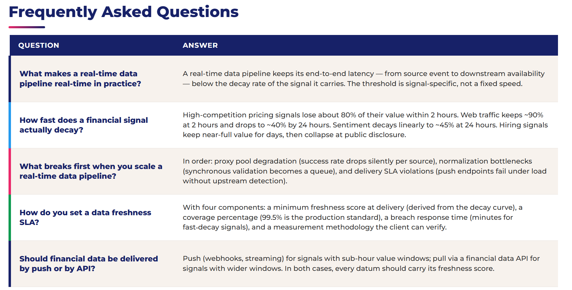
A real-time data pipeline is not one that extracts fast — it is one whose end-to-end latency stays below the decay rate of the signals it carries. In high-competition pricing categories, that window is under 2 hours. For hiring intelligence, the signal holds its value for days to weeks — until a public disclosure collapses it. The architecture has to match the signal, not a generic speed target.

This post goes a level deeper than our foundational guide, What Is Financial Data Scraping?, which covers the four alternative data signals that move investment decisions. Here the focus is on what happens inside the pipeline — and on the single metric that predicts whether a real-time data pipeline built on low-latency data extraction will hold up in production: freshness at the moment of delivery.

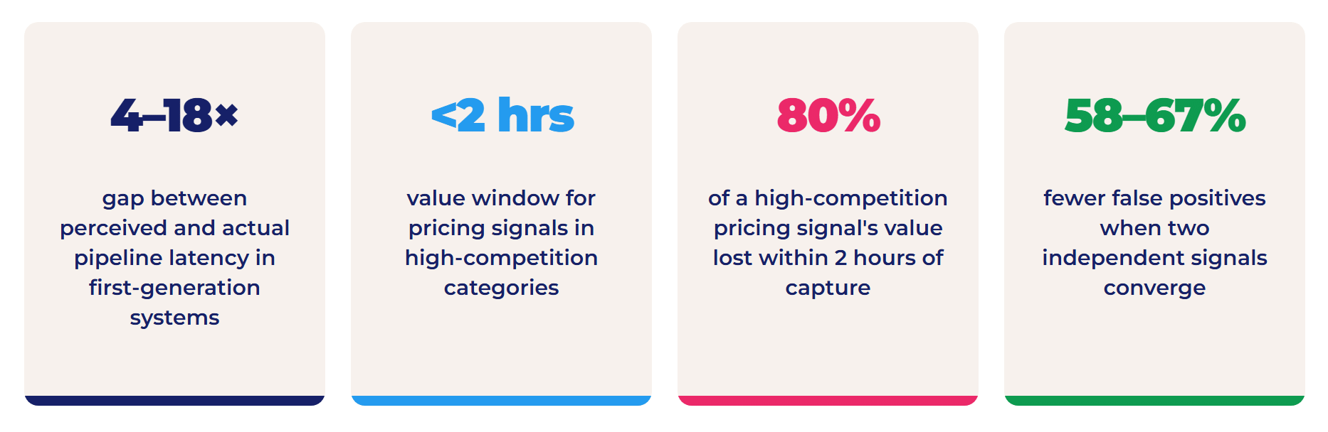
Source: Scraping Pros pipeline audit and deployment data, 2024–2026.

1. What Makes a Real-Time Data Pipeline Actually Real-Time?

Real-time is not a speed. It is a relationship: a real-time data pipeline is one whose end-to-end latency is lower than the decay rate of the signal it transports. A pipeline delivering pricing data in 4 hours is perfectly real-time for a long-horizon investment strategy. The same pipeline is useless for commodity arbitrage, where the action window is 12 minutes. “Real-time” is a property of the signal, not of the system.

Error #1: measuring extraction latency and calling it pipeline latency

This is the most common real-time data pipeline mistake. An 800 ms scrape looks fast. What rarely gets measured is the time between that 800 ms and the moment the normalized, validated, scored datum is available in the downstream decision system — which in unmonitored pipelines is routinely 30 to 90 minutes longer. Across Scraping Pros pipeline audits (2024–2026), effective end-to-end latency in first-generation systems runs 4 to 18 times higher than the extraction latency the engineering team believes it has. The gap lives in normalization queues, validation bottlenecks, and delivery stages that are never instrumented as a single unit.

The four latency regimes — and which one applies to alternative data

• Hard real-time (sub-second): guaranteed delivery within a fixed window, with system-level consequences if violated. Relevant for algorithmic trading execution; requires co-location and zero-copy memory management. Not the regime for alternative data strategies.
• Soft real-time (seconds to minutes): best-effort delivery within a threshold, with occasional violations tolerated. Relevant for live risk dashboards and position alerts. P99 latency matters more than the median.
• Near real-time (minutes to hours): delivery fast enough that the signal is still actionable before it decays. This is the operative regime for pricing intelligence, hiring signals, and sentiment monitoring — and the threshold is signal-specific.
• Micro-batch (hours to days): periodic aggregation windows. Often mislabeled as real-time. Sufficient for trend analysis; insufficient for event alerts.

Error #2: confusing polling frequency with data freshness

A system polling every 60 seconds does not have 60-second-fresh data. It has data that is up to 60 seconds stale in the best case — plus every downstream stage — with variable latency depending on when the source event occurred relative to the poll cycle. For discrete-event signals (a price change, a new job posting), trigger-based extraction outperforms polling at every frequency level. This is the core trade-off between batch scraping and a true streaming data architecture built on event platforms such as Apache Kafka.

2. The Freshness Decay Curve: How Fast Do Financial Signals Lose Value?

The Freshness Decay Curve plots the residual value of a financial signal — as a percentage of its value at capture — against time elapsed since capture. Each signal type has a distinct curve shape, and that shape sets the latency requirement of the real-time data pipeline carrying it. Get the curve wrong and you either over-engineer for signals with hours-long value windows, or under-engineer for signals that expire in minutes.

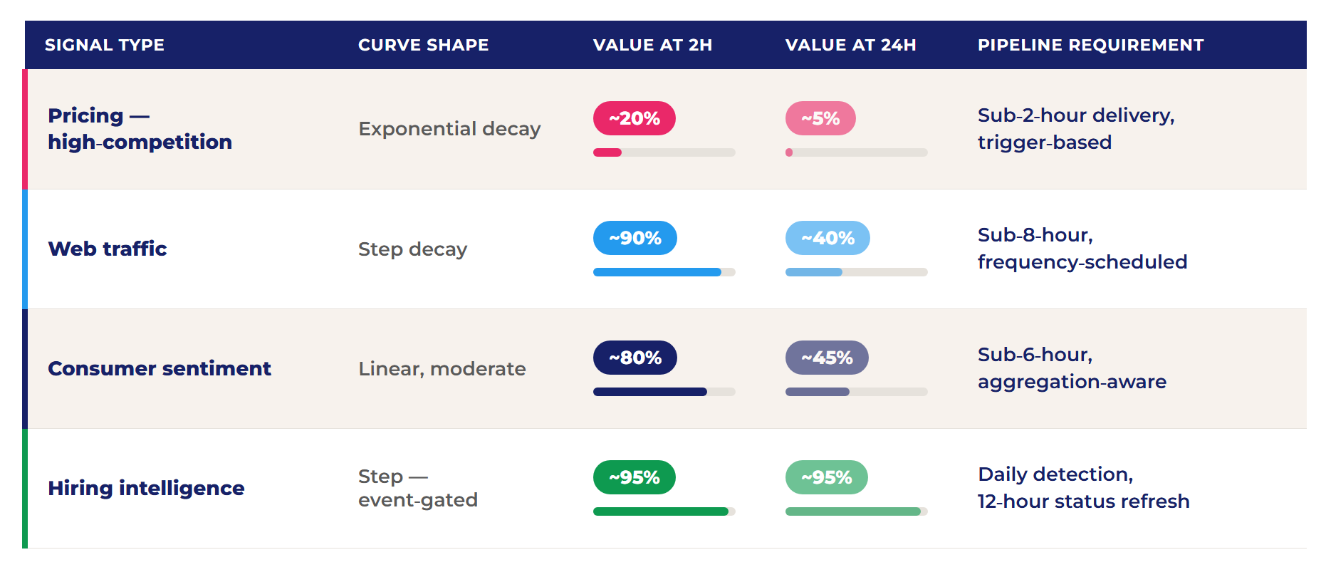
Source: Scraping Pros freshness decay analysis, 200+ monitored data sources, 2024–2026.

Pricing is the most demanding curve in the table — which is why e-commerce price monitoring at scale and autonomous pricing intelligence are built around trigger-based detection rather than fixed crawl schedules.

Why hiring signals need a different architecture

The hiring curve stays near 95% for days to weeks — but it does not decay gradually. It collapses abruptly when a public disclosure event occurs: the company announces the expansion, the job posting closes, or a published analysis makes the signal available to the broader market. For hiring data, the pipeline is not optimized for delivery speed. It is optimized for detection speed (finding the posting within 24 hours of publication) and status tracking (checking every 12 hours whether the posting is still active).

Convergence signals need parallel pipelines

Based on Scraping Pros deployment data, portfolios using convergence of two or more independent signal types — for example, hiring contraction and sentiment deterioration pointing in the same direction at the same time — reduced false-positive rates in their alternative data alerts by 58–67% compared to single-signal monitoring. The catch: the decay curves of those signals are different enough that each one needs its own pipeline configuration, running in parallel and joined only at the scoring layer. The same principle drives cross-industry AI scraping, where signals only become visible when you read across sources.

3. Real-Time Data Pipeline Reference Architecture: 4 Stages

Four stages. The first two are commonly implemented. The third — freshness scoring — is the component most frequently absent from first-generation pipelines, and its absence is what makes SLAs unverifiable. The fourth determines whether the architecture can sustain production load.

Stage 1: Ingestion

Two extraction patterns must coexist:

• Trigger-based for discrete-event signals: a price change, a new posting, a rating shift.
• Frequency-scheduled for continuous-flow signals: traffic metrics, aggregate sentiment.

The correct polling interval for scheduled extraction is not a default. It is calculated empirically from the observed change rate of each source during a 30–60 day calibration period. A source polled at 10× its actual change frequency is wasting 90% of its extraction capacity.

Two infrastructure components are systematically underspecified:

• Proxy pool management: pools must be segmented by source type, with success rate monitored per source. An aggregate 97% success rate can hide a critical source running at 70%.
• Anti-detection calibration: financial sources update their bot-detection logic continuously. A pipeline without a success-rate monitoring loop degrades silently.

Stage 2: Normalization

Three normalization dimensions are specific to financial data — and they are where investment-grade data is made or destroyed (see our approach to data cleaning and normalization):

• Entity resolution: the same company appears under different names, tickers, LEI codes, and ISIN codes across sources. All must resolve to one canonical entity before any cross-source analysis is possible.
• Timestamp separation: capture timestamp and publication timestamp must propagate as separate fields. They diverge significantly in high-latency sources, and collapsing them makes every freshness calculation downstream incorrect.
• Value normalization: prices, ratings, and counts appear in incompatible formats across markets. Normalization must be deterministic and auditable against the original captured value.

Stage 3: Freshness scoring

Every datum leaving the normalization layer receives a freshness score: a live percentage expressing how much of the signal’s original value remains, based on the calibrated decay curve for that source and signal type. The score does three jobs:

1. Routing: high-freshness data goes to real-time decision systems; low-freshness data goes to historical analysis.
2. Alerting: it triggers re-extraction or an SLA breach alert when a datum is projected to arrive below the minimum useful threshold.
3. Transparency: it travels with the datum as metadata, so downstream users know the actual freshness of every signal they consume.

Stage 4: Delivery and observability

Two delivery patterns: push (webhooks and streaming) for sub-hour signals, and pull (a financial data API) for wider value windows. Either way, the API must return the freshness score alongside the datum.

Four observability metrics must be instrumented and retained for at least 30 days:

• End-to-end latency distribution — not the mean. The P99 is what reveals production problems.
• Freshness score distribution at delivery.
• Extraction success rate per source.
• Normalization error rate.

A real-time data pipeline without these four metrics cannot be operated to an SLA. It can only be operated on hope.

4. What Breaks First When You Scale a Real-Time Data Pipeline?

Market data infrastructure rarely fails all at once. In Scraping Pros production deployments, failures appear in a predictable order:

1. Proxy pool degradation: success rate drops silently on specific sources while the aggregate number still looks healthy.
2. Normalization bottlenecks: synchronous validation that worked at 10 sources becomes a queue at 200 — and that queue is invisible latency.
3. Delivery SLA violations: push endpoints fail under load, and the failure is not detected upstream because nobody is measuring freshness at delivery.

Each failure maps to one of the four observability metrics above — which is why instrumenting them is a prerequisite, not an optimization. For teams deciding how much of this infrastructure to own, it is worth comparing managed scraping vs. DIY before scaling, and reviewing how serverless auto-scaling absorbs ingestion spikes.

5. How to Set a Data Freshness SLA That Means Something

The most common data freshness SLA in vendor contracts — “data will be updated every X minutes” — defines update frequency, not freshness. A system updating every 60 minutes with a 4-hour maintenance window has a contractual update frequency of 60 minutes and an effective maximum staleness of 5 hours. The SLA is met. The business requirement is not. Borrowing from Google’s SRE approach to service level objectives, the fix is to measure what the user actually experiences — here, freshness at delivery.

A commercially meaningful data freshness SLA has four components:

• Freshness threshold: the minimum freshness score acceptable at the moment of delivery, derived directly from the signal’s decay curve. If the curve shows 50% value at 6 hours and the use case requires at least 60%, the threshold implies a maximum of roughly 4.4 hours from capture to delivery on an exponential curve.
• Coverage: the percentage of monitored data that must meet the freshness threshold at any given time. In production financial data pipelines, 99.5% is the standard — no more than 0.5% of the monitored universe can sit below threshold without triggering a breach.
• Breach response time: the maximum time a datum can remain below threshold before the system raises an alert and starts a recovery action. Minutes for pricing signals; hours for hiring signals. Without this component, the SLA has no enforcement mechanism.
• Measurement methodology: how compliance is measured, how often, and who can see the data. An SLA that only the provider can measure is not verifiable. The pipeline must expose freshness metrics in real time through an API or client-accessible dashboard, with historical retention for audit.

Three questions must be answered before writing any number into a freshness SLA:

1. What is the freshness decay curve for this signal type?
2. What is the quantifiable business impact of consuming a datum at 60% freshness instead of 100%?
3. What does the system do automatically when it detects that a datum will breach the SLA before reaching its destination?

A real-time data pipeline that cannot answer the third question is not ready for production SLA commitments.

Action Items

• Measure end-to-end latency, not extraction latency: capture the source event timestamp and the downstream availability timestamp in your real-time data pipeline. The delta is your real latency. For most teams, this number is a surprise.
• Calibrate the freshness decay curve for your top three signals: use 90 days of historical data to correlate signal value with delivery latency retrospectively. That empirical curve is the input to every other architecture decision.
• Separate proxy pools by source type and monitor success rate per source: an aggregated success rate hides source-specific failures. Per-source monitoring is the minimum observability for a production pipeline.
• Add a freshness score as metadata on every delivered datum: even before you use it for routing, it tells analysts what fraction of each signal’s value they are actually consuming.
• Audit polling intervals against observed source change rates: if more than 60% of extraction cycles for a source return unchanged data, the interval is wrong and the capacity is wasted.
• Write the SLA with all four components: threshold, coverage, breach response time, and measurement methodology. If any of the four cannot be answered, the pipeline is not specified well enough for production commitments.